![\includegraphics[width=6cm]{TLpiece}](img20.png)
|
This section should derive the existence of the voltage and current waves on a transmission line. This way, it also proofs that the definitions from the last section make sense.
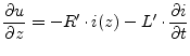
Figure 1.1 shows the equivalent circuit of an infinite
short piece of an arbitrary transmission line. The names of the
components all carry a single quotation mark which indicates a per-length
quantity. Thus, the units are ohms/m for ![]() , henry/m for
, henry/m for ![]() ,
siemens/m for
,
siemens/m for ![]() and farad/m for
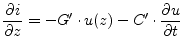
and farad/m for ![]() . Writing down the change of
voltage and current across a piece with length
. Writing down the change of
voltage and current across a piece with length
![]() results
in the transmission line equations.
results
in the transmission line equations.
 |
(1.5) |
 |
(1.6) |
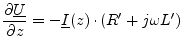
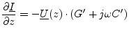
Transforming these equations into frequency domain leads to:
Taking equation 1.8 and setting it into the first derivative of equation 1.7 creates the wave equation:
 |
(1.9) |
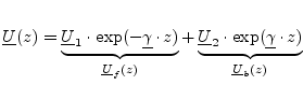
Note that both current waves are counted positive in positive ![]() direction.
In literature, the backward flowing current wave
direction.
In literature, the backward flowing current wave
![]() is
sometime counted the otherway around which would avoid the negative sign
within some of the following equations.
is
sometime counted the otherway around which would avoid the negative sign
within some of the following equations.
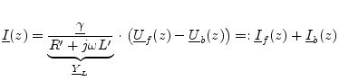
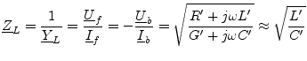
Equation 1.11 introduces the characteristic admittance
![]() . The propagation constant
. The propagation constant
![]() and the
characteristic impedance
and the
characteristic impedance
![]() are the two fundamental properties
describing a transmission line.
are the two fundamental properties
describing a transmission line.
 |
(1.12) |
Note that
![]() is a real value if the line loss (due to
is a real value if the line loss (due to
![]() and
and ![]() ) is small. This is often the case in reality.
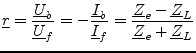
A further very important quantity is the reflexion coefficient
) is small. This is often the case in reality.
A further very important quantity is the reflexion coefficient
![]() which is defined as follows:
which is defined as follows:
 |
(1.13) |
The equation shows that a part of the voltage and current wave is reflected
back if the end of a transmission line is not terminated by an impedance
that equals
![]() . The same effect occurs in the middle of a
transmission line, if its characteristic impedance changes.
. The same effect occurs in the middle of a
transmission line, if its characteristic impedance changes.
|
|
|
|
|
|
|
|
|