| (15.58) |
When dealing with non-linear networks the number of equation systems to be solved depends on the required precision of the solution and the average necessary iterations until the solution is stable. This emphasizes the meaning of the solving procedures choice for different problems.
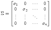
The equation systems
| (15.58) |
| (15.59) |
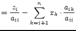
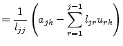
The elements
![]() of the inverse of the matrix
of the inverse of the matrix ![]() are
are
 |
(15.60) |
 |
using the |
(15.61) |
 |
using the |
(15.62) |
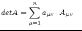
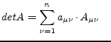
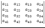
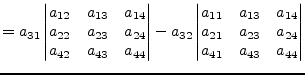
This method is called the Laplace expansion. In order to save
computing time the row or column with the most zeros in it is used for
the expansion expressed in the above equations. A sub determinant
![]() -th order of a matrix's element
-th order of a matrix's element
![]() of
of ![]() -th order is
the determinant which is computed by cancelling the
-th order is
the determinant which is computed by cancelling the ![]() -th row and
-th row and
![]() -th column. The following example demonstrates calculating the
determinant of a 4th order matrix with the elements of the 3rd row.
-th column. The following example demonstrates calculating the
determinant of a 4th order matrix with the elements of the 3rd row.
 |
 |
(15.63) |
 |
This recursive process for computing the inverse of a matrix is most
easiest to be implemented but as well the slowest algorithm. It
requires approximately ![]() operations.
operations.
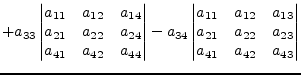
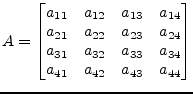
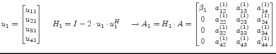
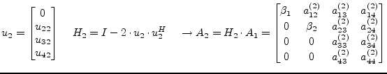
The Gaussian algorithm for solving a linear equation system is done in two parts: forward elimination and backward substitution. During forward elimination the matrix A is transformed into an upper triangular equivalent matrix. Elementary transformations due to an equation system having the same solutions for the unknowns as the original system.
 |
(15.64) |
The modifications applied to the matrix A in order to achieve this transformations are limited to the following set of operations.
The transformation of the matrix A is done in
![]() elimination steps. The new matrix elements of the k-th step with
elimination steps. The new matrix elements of the k-th step with
![]() are computed with the following
recursive formulas.
are computed with the following
recursive formulas.
| and |
(15.65) | |||
| and |
(15.66) | |||
| (15.67) |
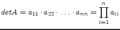
The triangulated matrix can be used to calculate the determinant very
easily. The determinant of a triangulated matrix is the product of
the diagonal elements. If the determinant ![]() is non-zero the
equation system has a solution. Otherwise the matrix A is singular.
is non-zero the
equation system has a solution. Otherwise the matrix A is singular.
 |
(15.68) |
When using row and/or column pivoting the resulting determinant may
differ in its sign and must be multiplied with ![]() whereas
whereas ![]() is
the number of row and column substitutions.
is
the number of row and column substitutions.
The Gaussian elimination fails if the pivot element ![]() turns to
be zero (division by zero). That is why row and/or column pivoting
must be used before each elimination step. If a diagonal element
turns to
be zero (division by zero). That is why row and/or column pivoting
must be used before each elimination step. If a diagonal element
![]() , then exchange the pivot row
, then exchange the pivot row ![]() with the row
with the row ![]() having the coefficient with the largest absolute value. The new pivot
row is
having the coefficient with the largest absolute value. The new pivot
row is ![]() and the new pivot element is going to be
and the new pivot element is going to be ![]() . If no
such pivot row can be found the matrix is singular.
. If no
such pivot row can be found the matrix is singular.
Total pivoting looks for the element with the largest absolute value within the matrix and exchanges rows and columns. When exchanging columns in equation systems the unknowns get reordered as well. For the numerical solution of equation systems with Gaussian elimination column pivoting is clever, and total pivoting recommended.
In order to improve numerical stability pivoting should also be
applied if
![]() because division by small diagonal elements
propagates numerical (rounding) errors. This appears especially with
poorly conditioned (the two dimensional case: two lines with nearly
the same slope) equation systems.
because division by small diagonal elements
propagates numerical (rounding) errors. This appears especially with
poorly conditioned (the two dimensional case: two lines with nearly
the same slope) equation systems.
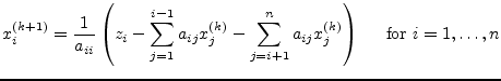
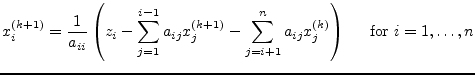
The solutions in the vector x are obtained by backward substituting into the triangulated matrix. The elements of the solution vector x are computed by the following recursive equations.
| (15.69) | |||
 |
(15.70) |
The forward elimination in the Gaussian algorithm requires
approximately ![]() , the backward substitution
, the backward substitution ![]() operations.
operations.
The Gauss-Jordan method is a modification of the Gaussian elimination. In each k-th elimination step the elements of the k-th column get zero except the diagonal element which gets 1. When the right hand side vector z is included in each step it contains the solution vector x afterwards.
The following recursive formulas must be applied to get the new matrix elements for the k-th elimination step. The k-th row must be computed first.
| (15.71) | |||
| (15.72) |
Then the other rows can be calculated with the following formulas.
| (15.73) | |||
| (15.74) |
Column pivoting may be necessary in order to avoid division by zero. The solution vector x is not harmed by row substitutions. When the Gauss-Jordan algorithm has been finished the original matrix has been transformed into the identity matrix. If each operation during this process is applied to an identity matrix the resulting matrix is the inverse matrix of the original matrix. This means that the Gauss-Jordan method can be used to compute the inverse of a matrix.
Though this elimination method is easy to implement the number of
required operations is larger than within the Gaussian elimination.
The Gauss-Jordan method requires approximately
![]() operations.
operations.
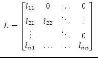
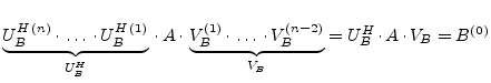
LU decomposition (decomposition into a lower and upper triangular matrix) is recommended when dealing with equation systems where the matrix A does not alter but the right hand side (the vector z) does. Both the Gaussian elimination and the Gauss-Jordan method involve both the right hand side and the matrix in their algorithm. Consecutive solutions of an equation system with an altering right hand side can be computed faster with LU decomposition.
The LU decomposition splits a matrix A into a product of a lower triangular matrix L with an upper triangular matrix U.
 and and 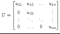 |
(15.75) |
The algorithm for solving the linear equation system ![]() involves
three steps:
involves
three steps:
The decomposition of the matrix A into a lower and upper triangular matrix is not unique. The most important decompositions, based on Gaussian elimination, are the Doolittle, the Crout and the Cholesky decomposition.
If pivoting is necessary during these algorithms they do not decompose
the matrix ![]() but the product with an arbitrary matrix
but the product with an arbitrary matrix ![]() (a
permutation of the matrix
(a
permutation of the matrix ![]() ). When exchanging rows and columns the
order of the unknowns as represented by the vector
). When exchanging rows and columns the
order of the unknowns as represented by the vector ![]() changes as well
and must be saved during this process for the forward substitution in
the algorithms second step.
changes as well
and must be saved during this process for the forward substitution in
the algorithms second step.
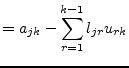
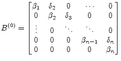
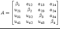
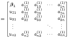
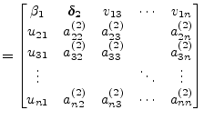
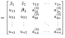
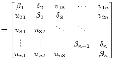
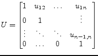
Using the decomposition according to Crout the coefficients of the L and U matrices can be stored in place the original matrix A. The upper triangular matrix U has the form
The diagonal elements ![]() are ones and thus the determinant
are ones and thus the determinant ![]() is one as well. The elements of the new coefficient matrix
is one as well. The elements of the new coefficient matrix ![]() for the k-th elimination step with
for the k-th elimination step with
![]() compute as
follows:
compute as
follows:
 |
(15.77) | |||
 |
(15.78) |
Pivoting may be necessary as you are going to divide by the diagonal
element ![]() .
.
The solutions in the arbitrary vector ![]() are obtained by forward
substituting into the triangulated
are obtained by forward
substituting into the triangulated ![]() matrix. At this stage you need
to remember the order of unknowns in the vector
matrix. At this stage you need
to remember the order of unknowns in the vector ![]() as changed by
pivoting. The elements of the solution vector
as changed by
pivoting. The elements of the solution vector ![]() are computed by the
following recursive equation.
are computed by the
following recursive equation.
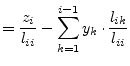 |
(15.79) |
The solutions in the vector ![]() are obtained by backward substituting
into the triangulated
are obtained by backward substituting
into the triangulated ![]() matrix. The elements of the solution vector
matrix. The elements of the solution vector
![]() are computed by the following recursive equation.
are computed by the following recursive equation.
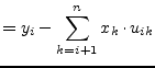 |
(15.80) |
The division by the diagonal elements of the matrix U is not necessary
because of Crouts definition in eq. (15.76) with
![]() .
.
The LU decomposition requires approximately
![]() operations for solving a linear equation system. For
operations for solving a linear equation system. For ![]() consecutive
solutions the method requires
consecutive
solutions the method requires
![]() operations.
operations.
Singular matrices actually having a solution are over- or
under-determined. These types of matrices can be handled by three
different types of decompositions: Householder, Jacobi (Givens
rotation) and singular value decomposition. Householder decomposition
factors a matrix ![]() into the product of an orthonormal matrix
into the product of an orthonormal matrix ![]() and
an upper triangular matrix
and
an upper triangular matrix ![]() , such that:
, such that:
| (15.81) |
The Householder decomposition is based on the fact that for any two
different vectors, ![]() and
and ![]() , with
, with
![]() , i.e. different vectors of equal length, a
reflection matrix
, i.e. different vectors of equal length, a
reflection matrix ![]() exists such that:
exists such that:
| (15.82) |
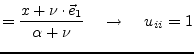
To obtain the matrix ![]() , the vector
, the vector ![]() is defined by:
is defined by:
| (15.83) |
The matrix ![]() defined by
defined by
is then the required reflection matrix.
The equation system
| (15.85) |
With
![]() this yields
this yields
| (15.86) |
Since ![]() is triangular the equation system is solved by a simple
matrix-vector multiplication on the right hand side and backward
substitution.
is triangular the equation system is solved by a simple
matrix-vector multiplication on the right hand side and backward
substitution.
Starting with ![]() , let
, let ![]() = the first column of
= the first column of ![]() , and
, and
![]() , i.e. a column
vector whose first component is the norm of
, i.e. a column
vector whose first component is the norm of ![]() with the remaining
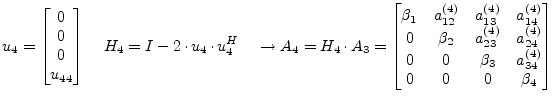
components equal to 0. The Householder transformation
with the remaining
components equal to 0. The Householder transformation
![]() with
with
![]() will turn the first column of
will turn the first column of ![]() into
into ![]() as with
as with
![]() . At each stage
. At each stage ![]() ,
, ![]() = the kth column of
= the kth column of ![]() on and below the diagonal with all other components equal to 0, and
on and below the diagonal with all other components equal to 0, and
![]() 's kth component equals the norm of
's kth component equals the norm of ![]() with all other
components equal to 0. Letting
with all other
components equal to 0. Letting
![]() , the
components of the kth column of
, the
components of the kth column of ![]() below the diagonal are each
0. These calculations are listed below for each stage for the matrix
A.
below the diagonal are each
0. These calculations are listed below for each stage for the matrix
A.
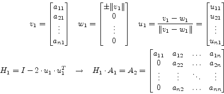 |
(15.87) |
With this first step the upper left diagonal element of the ![]() matrix,
matrix,
![]() , has been generated. The
elements below are zeroed out. Since
, has been generated. The
elements below are zeroed out. Since ![]() can be generated from
can be generated from
![]() stored in place of the first column of
stored in place of the first column of ![]() the multiplication
the multiplication
![]() can be performed without actually generating
can be performed without actually generating ![]() .
.
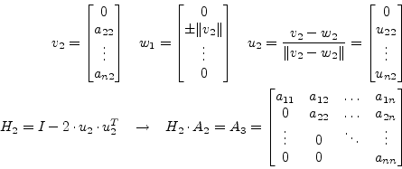 |
(15.88) |
These elimination steps generate the ![]() matrix because
matrix because ![]() is
orthonormal, i.e.
is
orthonormal, i.e.
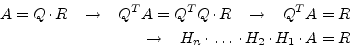 |
(15.89) |
After ![]() elimination steps the original matrix
elimination steps the original matrix ![]() contains the upper
triangular matrix
contains the upper
triangular matrix ![]() , except for the diagonal elements which can be
stored in some vector. The lower triangular matrix contains the
Householder vectors
, except for the diagonal elements which can be
stored in some vector. The lower triangular matrix contains the
Householder vectors
![]() .
.
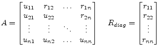 |
(15.90) |
With
![]() this representation
contains both the
this representation
contains both the ![]() and
and ![]() matrix, in a packed form, of course:
matrix, in a packed form, of course: ![]() as a composition of Householder vectors and
as a composition of Householder vectors and ![]() in the upper
triangular part and its diagonal vector
in the upper
triangular part and its diagonal vector ![]() .
.
In order to form the right hand side ![]() let remember
eq. (15.84) denoting the reflection matrices used
to compute
let remember
eq. (15.84) denoting the reflection matrices used
to compute ![]() .
.
| (15.91) |
Thus it is possible to replace the original right hand side vector ![]() by
by
| (15.92) |
which yields for each
![]() the following expression:
the following expression:
The latter
![]() is a simple scalar product of two vectors.
Performing eq. (15.93) for each Householder vector finally
results in the new right hand side vector
is a simple scalar product of two vectors.
Performing eq. (15.93) for each Householder vector finally
results in the new right hand side vector ![]() .
.
The solutions in the vector ![]() are obtained by backward substituting
into the triangulated
are obtained by backward substituting
into the triangulated ![]() matrix. The elements of the solution vector
matrix. The elements of the solution vector
![]() are computed by the following recursive equation.
are computed by the following recursive equation.
 |
(15.94) |
Though the QR decomposition has an operation count of
![]() (which is about six times more than the LU decomposition) it has its
advantages. The QR factorization method is said to be unconditional
stable and more accurate. Also it can be used to obtain the
minimum-norm (or least square) solution of under-determined equation
systems.
(which is about six times more than the LU decomposition) it has its
advantages. The QR factorization method is said to be unconditional
stable and more accurate. Also it can be used to obtain the
minimum-norm (or least square) solution of under-determined equation
systems.
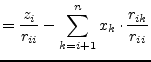
The circuit in fig. 15.3 has the following MNA representation:
 |
(15.95) |
The second and third row of the matrix ![]() are linear dependent and
the matrix is singular because its determinant is zero. Depending on
the right hand side
are linear dependent and
the matrix is singular because its determinant is zero. Depending on
the right hand side ![]() , the equation system has none or unlimited
solutions. This is called an under-determined system. The discussed
QR decomposition easily computes a valid solution without reducing
accuracy. The LU decomposition would probably fail because of the
singularity.
, the equation system has none or unlimited
solutions. This is called an under-determined system. The discussed
QR decomposition easily computes a valid solution without reducing
accuracy. The LU decomposition would probably fail because of the
singularity.
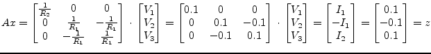
With some more effort it is possible to obtain the minimum-norm solution of this problem. The algorithm as described here would probably yield the following solution:
 |
(15.96) |
This is one out of unlimited solutions. The following short description shows how it is possible to obtain the minimum-norm solution. When decomposing the transposed problem
| (15.97) |
the minimum-norm solution ![]() is obtained by forward substitution of
is obtained by forward substitution of
| (15.98) |
and multiplying the result with ![]() .
.
| (15.99) |
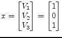
In the example above this algorithm results in a solution vector with the least vector norm possible:
 |
(15.100) |
This algorithm outline is also sometimes called LQ decomposition
because of ![]() being a lower triangular matrix used by the forward
substitution.
being a lower triangular matrix used by the forward
substitution.
Very bad conditioned (ratio between largest and smallest eigenvalue) matrices, i.e. nearly singular, or even singular matrices (over- or under-determined equation systems) can be handled by the singular value decomposition (SVD). This type of decomposition is defined by
where the ![]() matrix consists of the orthonormalized eigenvectors
associated with the eigenvalues of
matrix consists of the orthonormalized eigenvectors
associated with the eigenvalues of
![]() ,
, ![]() consists of the
orthonormalized eigenvectors of
consists of the
orthonormalized eigenvectors of
![]() and
and ![]() is a matrix
with the singular values of
is a matrix
with the singular values of ![]() (non-negative square roots of the
eigenvalues of
(non-negative square roots of the
eigenvalues of
![]() ) on its diagonal and zeros otherwise.
) on its diagonal and zeros otherwise.
 |
(15.102) |
The singular value decomposition can be used to solve linear equation systems by simple substitutions
| (15.103) | ||
| (15.104) | ||
| (15.105) |
| (15.106) |
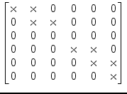
To obtain the decomposition stated in eq. (15.101) Householder
vectors are computed and their transformations are applied from the
left-hand side and right-hand side to obtain an upper bidiagonal
matrix ![]() which has the same singular values as the original
which has the same singular values as the original ![]() matrix because all of the transformations introduced are orthogonal.
matrix because all of the transformations introduced are orthogonal.
| (15.107) |
Specifically,
![]() annihilates the subdiagonal elements in
column
annihilates the subdiagonal elements in
column ![]() and
and ![]() zeros out the appropriate elements in row
zeros out the appropriate elements in row
![]() .
.
 |
(15.108) |
Afterwards an iterative process (which turns out to be a QR iteration)
is used to transform the bidiagonal matrix ![]() into a diagonal form by
applying successive Givens transformations (therefore orthogonal as
well) to the bidiagonal matrix. This iteration is said to have cubic
convergence and yields the final singular values of the matrix
into a diagonal form by
applying successive Givens transformations (therefore orthogonal as
well) to the bidiagonal matrix. This iteration is said to have cubic
convergence and yields the final singular values of the matrix ![]() .
.
| (15.109) |
 |
(15.110) |
Each of the transformations applied to the bidiagonal matrix is also
applied to the matrices ![]() and
and ![]() which finally yield the
which finally yield the ![]() and
and ![]() matrices after convergence.
matrices after convergence.
So far for the algorithm outline. Without the very details the following sections briefly describe each part of the singular value decomposition.
Beforehand some notation marks are going to be defined.
 |
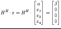
A Householder matrix is an elementary unitary matrix that is
Hermitian. Its fundamental use is their ability to transform a vector
![]() to a multiple of
to a multiple of ![]() , the first column of the identity
matrix. The elementary Hermitian (i.e. the Householder matrix) is
defined as
, the first column of the identity
matrix. The elementary Hermitian (i.e. the Householder matrix) is
defined as
| (15.111) |
Beside excellent numerical properties, their application demonstrates
their efficiency. If ![]() is a matrix, then
is a matrix, then
| (15.112) | ||
In order to reduce a 4![]() 4 matrix
4 matrix ![]() to upper triangular form
successive Householder reflectors must be applied.
to upper triangular form
successive Householder reflectors must be applied.
 |
(15.113) |
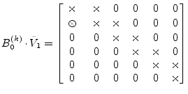
In the first step the diagonal element ![]() gets replaced and its
below elements get annihilated by the multiplication with an
appropriate Householder vector, also the remaining right-hand columns
get modified.
gets replaced and its
below elements get annihilated by the multiplication with an
appropriate Householder vector, also the remaining right-hand columns
get modified.
 |
(15.114) |
This process must be repeated
 |
(15.115) |
 |
(15.116) |
 |
(15.117) |
until the matrix ![]() contains an upper triangular matrix
contains an upper triangular matrix ![]() . The
matrix
. The
matrix ![]() can be expressed as the the product of the Householder
vectors. The performed operations deliver
can be expressed as the the product of the Householder
vectors. The performed operations deliver
| (15.118) |
since ![]() is unitary. The matrix
is unitary. The matrix ![]() itself can be expressed in terms
of
itself can be expressed in terms
of ![]() using the following transformation.
using the following transformation.
The eqn. (15.119)-(15.121) are necessary to be mentioned
only in case ![]() is not Hermitian, but still unitary. Otherwise there
is no difference computing
is not Hermitian, but still unitary. Otherwise there
is no difference computing ![]() or
or ![]() using the Householder vectors.
No care must be taken in choosing forward or backward accumulation.
using the Householder vectors.
No care must be taken in choosing forward or backward accumulation.
In the general case it is necessary to find an elementary unitary matrix
| (15.122) |
When choosing the elements
![]() it is possible the store the
Householder vectors as well as the upper triangular matrix
it is possible the store the
Householder vectors as well as the upper triangular matrix ![]() in the
same storage of the matrix
in the
same storage of the matrix ![]() . The Householder matrices
. The Householder matrices ![]() can be
completely restored from the Householder vectors.
can be
completely restored from the Householder vectors.
 |
(15.124) |
There exist several approaches to meet the conditions expressed in
eq. (15.123). For fewer computational effort it may be
convenient to choose ![]() to be real valued. With the notation
to be real valued. With the notation
 |
(15.125) |
one possibility is to define the following calculation rules.
| (15.126) | ||
| (15.127) | ||
| (15.128) | ||
| (15.129) | ||
 |
(15.130) |
These definitions yield a complex ![]() , thus
, thus ![]() is no more
Hermitian but still unitary.
is no more
Hermitian but still unitary.
| (15.131) |
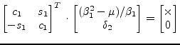
A Givens rotation is a plane rotation matrix. Such a plane rotation matrix is an orthogonal matrix that is different from the identity matrix only in four elements.
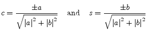
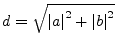
The elements are usually chosen so that
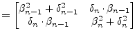
The most common use of such a plane rotation is to choose ![]() and
and ![]() such that for a given
such that for a given ![]() and
and ![]()
 |
(15.135) |
 |
(15.136) |
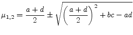
The eigenvalues of a 2-by-2 matrix
 |
(15.137) |
can be obtained directly from the quadratic formula. The characteristic polynomial is
 |
(15.138) |
The polynomial yields the two eigenvalues.
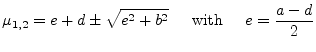
For a symmetric matrix ![]() (i.e.
(i.e. ![]() ) eq.(15.139) can
be rewritten to:
) eq.(15.139) can
be rewritten to:
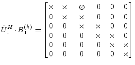
In the first step the original matrix ![]() is bidiagonalized by the
application of Householder reflections from the left and right hand
side. The matrices
is bidiagonalized by the
application of Householder reflections from the left and right hand
side. The matrices ![]() and
and ![]() can each be determined as a
product of Householder matrices.
can each be determined as a
product of Householder matrices.
 |
(15.141) |
Each of the required Householder vectors are created and applied as
previously defined. Suppose a ![]() matrix, then applying the
first Householder vector from the left hand side eliminates the first
column and yields
matrix, then applying the
first Householder vector from the left hand side eliminates the first
column and yields
 |
(15.142) | |
|
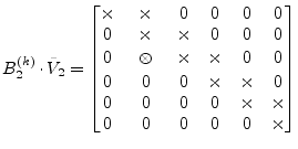
Next, a Householder vector is applied from the right hand side to annihilate the first row.
| ||
 |
(15.143) | |
|
Again, a Householder vector is applied from the left hand side to annihilate the second column.
| ||
 |
(15.144) | |
|
This process is continued until
| ||
 |
(15.145) | |
For each of the Householder transformations from the left and right
hand side the appropriate ![]() values must be stored in separate
vectors.
values must be stored in separate
vectors.
Using the Householder vectors stored in place of the original ![]() matrix and the appropriate
matrix and the appropriate ![]() value vectors it is now necessary to
unpack the
value vectors it is now necessary to
unpack the ![]() and
and ![]() matrices. The diagonal vector
matrices. The diagonal vector ![]() and the super-diagonal vector
and the super-diagonal vector ![]() can be saved in separate
vectors previously. Thus the
can be saved in separate
vectors previously. Thus the ![]() matrix can be unpacked in place of
the
matrix can be unpacked in place of
the ![]() matrix and the
matrix and the ![]() matrix is unpacked in a separate
matrix.
matrix is unpacked in a separate
matrix.
There are two possible algorithms for computing the Householder product matrices, i.e. forward accumulation and backward accumulation. Both start with the identity matrix which is successively multiplied by the Householder matrices either from the left or right.
| (15.146) | ||
| (15.147) |
Recall that the leading portion of each Householder matrix is the
identity except the first. Thus, at the beginning of backward
accumulation, ![]() is ``mostly the identity'' and it gradually
becomes full as the iteration progresses. This pattern can be
exploited to reduce the number of required flops. In contrast,
is ``mostly the identity'' and it gradually
becomes full as the iteration progresses. This pattern can be
exploited to reduce the number of required flops. In contrast,
![]() is full in forward accumulation after the first step. For
this reason, backward accumulation is cheaper and the strategy of
choice. When unpacking the
is full in forward accumulation after the first step. For
this reason, backward accumulation is cheaper and the strategy of
choice. When unpacking the ![]() matrix in place of the original
matrix in place of the original ![]() matrix it is necessary to choose backward accumulation anyway.
matrix it is necessary to choose backward accumulation anyway.
| (15.148) | ||
| (15.149) |
Unpacking the ![]() matrix is done in a similar way also performing
successive Householder matrix multiplications using backward
accumulation.
matrix is done in a similar way also performing
successive Householder matrix multiplications using backward
accumulation.
At this stage the matrices ![]() and
and ![]() exist in unfactored form.
Also there are the diagonal vector
exist in unfactored form.
Also there are the diagonal vector ![]() and the super-diagonal
vector
and the super-diagonal
vector ![]() . Both vectors are real valued. Thus the following
algorithm can be applied even though solving a complex equation
system.
. Both vectors are real valued. Thus the following
algorithm can be applied even though solving a complex equation
system.
|
(15.150) |
The remaining problem is thus to compute the SVD of the matrix ![]() .
This is done applying an implicit-shift QR step to the tridiagonal
matrix
.
This is done applying an implicit-shift QR step to the tridiagonal
matrix ![]() which is a symmetric. The matrix
which is a symmetric. The matrix ![]() is not
explicitly formed that is why a QR iteration with implicit shifts is
applied.
is not
explicitly formed that is why a QR iteration with implicit shifts is
applied.
After bidiagonalization we have a bidiagonal matrix ![]() :
:
| (15.151) |
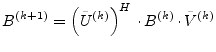
The presented method turns ![]() into a matrix
into a matrix ![]() by
applying a set of orthogonal transforms
by
applying a set of orthogonal transforms
The orthogonal matrices ![]() and
and ![]() are chosen so that
are chosen so that
![]() is also a bidiagonal matrix, but with the super-diagonal
elements smaller than those of
is also a bidiagonal matrix, but with the super-diagonal
elements smaller than those of ![]() . The eq.(15.152)
is repeated until the non-diagonal elements of
. The eq.(15.152)
is repeated until the non-diagonal elements of ![]() become
smaller than
become
smaller than
![]() and can be disregarded.
and can be disregarded.
The matrices ![]() and
and ![]() are constructed as
are constructed as
| (15.153) |
and similarly ![]() where
where
![]() and
and
![]() are
matrices of simple rotations as given in eq.(15.132). Both
are
matrices of simple rotations as given in eq.(15.132). Both
![]() and
and ![]() are products of Givens rotations and thus
perform orthogonal transforms.
are products of Givens rotations and thus
perform orthogonal transforms.
The left multiplication of ![]() by
by
![]() replaces two
rows of
replaces two
rows of ![]() by their linear combinations. The rest of
by their linear combinations. The rest of ![]() is unaffected. Right multiplication of
is unaffected. Right multiplication of ![]() by
by
![]() similarly changes only two columns of
similarly changes only two columns of ![]() .
.
A matrix
![]() is chosen the way that
is chosen the way that
| (15.154) |
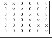
is a QR transform with a shift. Note that multiplying ![]() by
by
![]() gives rise to a non-zero element which is below the main
diagonal.
gives rise to a non-zero element which is below the main
diagonal.
 |
(15.155) |
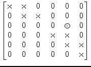
A new rotation angle is then chosen so that multiplication by
![]() gets rid of that element. But this will create a
non-zero element which is right beside the super-diagonal.
gets rid of that element. But this will create a
non-zero element which is right beside the super-diagonal.
 |
(15.156) |
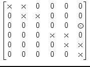
Then
![]() is made to make it disappear, but this leads to
another non-zero element below the diagonal, etc.
is made to make it disappear, but this leads to
another non-zero element below the diagonal, etc.
 |
(15.157) |
In the end, the matrix
![]() becomes bidiagonal
again. However, because of a special choice of
becomes bidiagonal
again. However, because of a special choice of
![]() (QR
algorithm), its non-diagonal elements are smaller than those of
(QR
algorithm), its non-diagonal elements are smaller than those of ![]() .
.
Please note that each of the transforms must also be applied to the
unfactored ![]() and
and ![]() matrices which turns them successively
into
matrices which turns them successively
into ![]() and
and ![]()
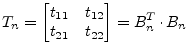
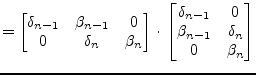
For a single QR step the computation of the eigenvalue ![]() of the
trailing 2-by-2 submatrix of
of the
trailing 2-by-2 submatrix of
![]() that is closer to
the
that is closer to
the ![]() matrix element is required.
matrix element is required.
 |
 |
(15.158) |
 |
(15.159) |
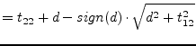
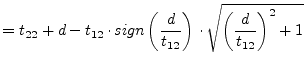
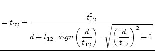
The required eigenvalue is called Wilkinson shift, see
eq.(15.140) for details. The sign for the eigenvalue
is chosen such that it is closer to ![]() .
.
 |
(15.160) | |
 |
(15.161) | |
 |
(15.162) |
| (15.163) |
The Givens rotation
![]() is chosen such that
is chosen such that
 |
(15.164) |
The special choice of this first rotation in the single QR step
ensures that the super-diagonal matrix entries get smaller.
Typically, after a few of these QR steps, the super-diagonal entry
![]() becomes negligible.
becomes negligible.
The QR iteration described above claims to hold if the underlying bidiagonal matrix is unreduced, i.e. has no zeros neither on the diagonal nor on the super-diagonal.
When there is a zero along the diagonal, then premultiplication by a
sequence of Givens transformations can zero the right-hand
super-diagonal entry as well. The inverse rotations must be applied
to the ![]() matrix.
matrix.
 |
 |
|||
 |
 |
Thus the problem can be decoupled into two smaller matrices ![]() and
and
![]() . The diagonal matrix
. The diagonal matrix ![]() is successively getting larger for
each super-diagonal entry being neglected after the QR iterations.
is successively getting larger for
each super-diagonal entry being neglected after the QR iterations.
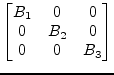 |
(15.165) |
Matrix ![]() has non-zero super-diagonal entries. If there is any
zero diagonal entry in
has non-zero super-diagonal entries. If there is any
zero diagonal entry in ![]() , then the super-diagonal entry can be
annihilated as just described. Otherwise the QR iteration algorithm
can be applied to
, then the super-diagonal entry can be
annihilated as just described. Otherwise the QR iteration algorithm
can be applied to ![]() .
.
When there are only ![]() matrix entries left (diagonal entries only)
the algorithm is finished, then the
matrix entries left (diagonal entries only)
the algorithm is finished, then the ![]() matrix has been transformed
into the singular value matrix
matrix has been transformed
into the singular value matrix ![]() .
.
It is straight-forward to solve a given equation system once having the singular value decomposition computed.
| (15.166) | ||
| (15.167) | ||
| (15.168) | ||
| (15.169) | ||
| (15.170) |
The inverse of the diagonal matrix ![]() yields
yields
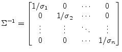 |
(15.171) |
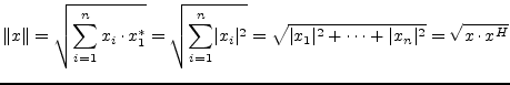
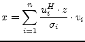
With ![]() being the i-th row of the matrix
being the i-th row of the matrix ![]() ,
, ![]() the i-th column
of the matrix
the i-th column
of the matrix ![]() and
and ![]() the i-th singular value
eq. (15.170) can be rewritten to
the i-th singular value
eq. (15.170) can be rewritten to
 |
(15.172) |
It must be mentioned that very small singular values ![]() corrupt the complete result. Such values indicate (nearly) singular
(ill-conditioned) matrices
corrupt the complete result. Such values indicate (nearly) singular
(ill-conditioned) matrices ![]() . In such cases, the solution vector
. In such cases, the solution vector
![]() obtained by zeroing the small
obtained by zeroing the small ![]() 's and then using equation
(15.170) is better than direct-method solutions (such
as LU decomposition or Gaussian elimination) and the SVD solution
where the small
's and then using equation
(15.170) is better than direct-method solutions (such
as LU decomposition or Gaussian elimination) and the SVD solution
where the small ![]() 's are left non-zero. It may seem
paradoxical that this can be so, since zeroing a singular value
corresponds to throwing away one linear combination of the set of
equations that is going to be solved. The resolution of the paradox
is that a combination of equations that is so corrupted by roundoff
error is thrown away precisely as to be at best useless; usually it is
worse than useless since it "pulls" the solution vector way off
towards infinity along some direction that is almost a nullspace
vector.
's are left non-zero. It may seem
paradoxical that this can be so, since zeroing a singular value
corresponds to throwing away one linear combination of the set of
equations that is going to be solved. The resolution of the paradox
is that a combination of equations that is so corrupted by roundoff
error is thrown away precisely as to be at best useless; usually it is
worse than useless since it "pulls" the solution vector way off
towards infinity along some direction that is almost a nullspace
vector.
This method quite simply involves rearranging each equation to make
each variable a function of the other variables. Then make an initial
guess for each solution and iterate. For this method it is necessary
to ensure that all the diagonal matrix elements ![]() are non-zero.
This is given for the nodal analysis and almostly given for the
modified nodal analysis. If the linear equation system is solvable
this can always be achieved by rows substitutions.
are non-zero.
This is given for the nodal analysis and almostly given for the
modified nodal analysis. If the linear equation system is solvable
this can always be achieved by rows substitutions.
The algorithm for performing the iteration step ![]() writes as
follows.
writes as
follows.
 |
(15.173) |
This has to repeated until the new solution vectors ![]() deviation from the previous one
deviation from the previous one ![]() is sufficiently small.
is sufficiently small.
The initial guess has no effect on whether the iterative method converges or not, but with a good initial guess (as possibly given in consecutive Newton-Raphson iterations) it converges faster (if it converges). To ensure convergence the condition
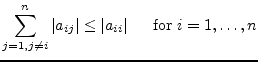 |
(15.174) |
and at least one case
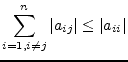 |
(15.175) |
must apply. If these conditions are not met, the iterative equations may still converge. If these conditions are met the iterative equations will definitely converge.
Another simple approach to a convergence criteria for iterative algorithms is the Schmidt and v. Mises criteria.
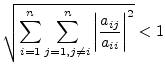 |
(15.176) |
The Gauss-Seidel algorithm is a modification of the Jacobi method. It uses the previously computed values in the solution vector of the same iteration step. That is why this iterative method is expected to converge faster than the Jacobi method.
The slightly modified algorithm for performing the ![]() iteration
step writes as follows.
iteration
step writes as follows.
 |
(15.177) |
The remarks about the initial guess ![]() as well as the
convergence criteria noted in the section about the Jacobi method
apply to the Gauss-Seidel algorithm as well.
as well as the
convergence criteria noted in the section about the Jacobi method
apply to the Gauss-Seidel algorithm as well.
There are direct and iterative methods (algorithms) for solving linear equation systems. Equation systems with large and sparse matrices should rather be solved with iterative methods.
| method |
precision |
application |
programming effort |
computing complexity |
notes
|
| Laplace expansion |
numerical errors |
general |
straight forward |
|
very time consuming
|
| Gaussian elimination |
numerical errors |
general |
intermediate |
|
|
| Gauss-Jordan |
numerical errors |
general |
intermediate |
|
computes the inverse besides
|
| LU decomposition |
numerical errors |
general |
intermediate |
|
useful for consecutive solutions
|
| QR decomposition |
good |
general |
high |
|
|
| Singular value decomposition |
good |
general |
very high |
|
ill-conditioned matrices can be handled
|
| Jacobi |
very good |
diagonally dominant systems |
easy |
|
possibly no convergence
|
| Gauss-Seidel |
very good |
diagonally dominant systems |
easy |
|
possibly no convergence
|
![\includegraphics[width=10cm]{MNAsingular}](img2894.png)
![$\displaystyle M = \left[ \begin{array}{ccccccccccc} 1 & 0 & \cdots & & & & & & ...
... & & & \ddots & 0\\ 0 & \cdots & & & & & & & \cdots & 0 & 1 \end{array} \right]$](img2961.png)
![$\displaystyle R = \left[\begin{array}{rl} c & s\\ -s & c\\ \end{array}\right] \...
... \rightarrow \;\;\;\; \left\vert c\right\vert^2 + \left\vert s\right\vert^2 = 1$](img2962.png)
![$\displaystyle R = \left[\begin{array}{rl} c & s\\ -s & c\\ \end{array}\right] \cdot \begin{bmatrix}a\\ b\\ \end{bmatrix} = \begin{bmatrix}d\\ 0\\ \end{bmatrix}$](img2963.png)