Noise Wave Correlation Matrix in CAE

Due to the similar concept of S parameters and noise correlation coefficients, the CAE noise analysis can be performed quite alike the S parameter analysis (section 1.3.1). As each step uses the S parameters to calculate the noise correlation matrix, the noise analysis is best done step by step in parallel with the S parameter analysis. Performing each step is as follows: We have the noise wave correlation matrices ( $(\underline{C})$, $(\underline{D})$ ) and the S parameter matrices ( $(\underline{S})$, $(\underline{T})$ ) of two arbitrary circuits and want to know the correlation matrix of the special circuit resulting from connecting two circuits at one port.

Figure 2.2: connecting two noisy circuits, scheme (left) and signal flow graph (right)

An example is shown in fig. 2.2. What we have to do is to transform the inner noise waves $\underline{b}_{noise,k}$ and $\underline{b}_{noise,l}$ to the open ports. Let us look upon the example. According to the signal flow graph the resulting noise wave $\underline{b}_{noise,i}'$ writes as follows:

$$\underline{b}_{noise,i}' = \underline{b}_{noise,i} + \underline{b... ...,l}\cdot \frac{\underline{S}_{ik}}{1-\underline{S}_{kk}\cdot\underline{T}_{ll}}$$ (2.25)

The noise wave $\underline{b}_{noise,j}$ does not contribute to $\underline{b}_{noise,i}'$, because no path leads to port $i$. Calculating $\underline{b}_{noise,j}'$ is quite alike:

$$\underline{b}_{noise,j}' = \underline{b}_{noise,j} + \underline{b... ...,k}\cdot \frac{\underline{T}_{jl}}{1-\underline{S}_{kk}\cdot\underline{T}_{ll}}$$ (2.26)

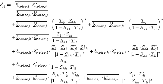
Now we can derive the first element of the new noise correlation matrix by multiplying eq. (2.25) with eq. (2.26).

$$\begin{split}\underline{c}_{ij}' = & \quad \overline{\underli... ...-\underline{S}_{kk}\cdot\underline{T}_{ll} \vert^2} \end{split}$$ (2.27)

The noise waves of different circuits are uncorrelated and therefore their time average product equals zero (e.g. $\overline{\underline{b}_{noise,i}\cdot\underline{b}_{noise,j}^*} = 0$). Thus, the final result is:

$$\begin{split}\underline{c}_{ij}' = (\underline{c}_{ji}')^* = ... ..._{ik}}{1-\underline{S}_{kk}\cdot\underline{T}_{ll}} \end{split}$$ (2.28)

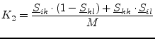
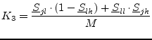
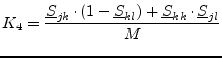
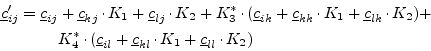
All other cases of connecting circuits can be calculated the same way using the signal flow graph. The results are listed below.

If index $i$ and $j$ are within the same circuit, it results in fig. 2.3. The following formula holds:

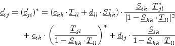
$$\begin{split}\underline{c}_{ij}' = (\underline{c}_{ji}')^* = ... ..._{ik}}{1-\underline{S}_{kk}\cdot\underline{T}_{ll}} \end{split}$$ (2.29)

This equation is also valid, if $i$ equals $j$.

Figure 2.3: connecting two noisy circuits

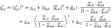
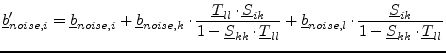
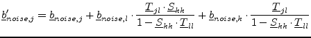
If the connected ports $k$ and $l$ are from the same circuit, the following equations must be applied (see also fig. 2.4) to obtain the new correlation matrix coefficients.

$$M = (1-\underline{S}_{kl})\cdot(1-\underline{S}_{lk}) - \underline{S}_{kk}\cdot\underline{S}_{ll}$$ (2.30)

$$K_1 = \frac{\underline{S}_{il}\cdot(1-\underline{S}_{lk}) + \underline{S}_{ll}\cdot\underline{S}_{ik}} {M}$$ (2.31)

$$K_2 = \frac{\underline{S}_{ik}\cdot(1-\underline{S}_{kl}) + \underline{S}_{kk}\cdot\underline{S}_{il}} {M}$$ (2.32)

$$K_3 = \frac{\underline{S}_{jl}\cdot(1-\underline{S}_{lk}) + \underline{S}_{ll}\cdot\underline{S}_{jk}} {M}$$ (2.33)

$$K_4 = \frac{\underline{S}_{jk}\cdot(1-\underline{S}_{kl}) + \underline{S}_{kk}\cdot\underline{S}_{jl}} {M}$$ (2.34)

$$\begin{split}\underline{c}_{ij}' = \underline{c}_{ij} &+ \und... ...ine{c}_{kl}\cdot K_1 + \underline{c}_{ll}\cdot K_2) \end{split}$$ (2.35)

These equations are also valid if $i$ equals $j$.

Figure 2.4: connection within a noisy circuits

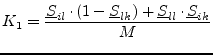
The absolute values of the noise correlation coefficients are very small. To achieve a higher numerical precision, it is recommended to normalize the noise matrix with $k\cdot T_0$. After the simulation they do not have to be denormalized, because the noise parameters can be calculated by using equation (2.4) to (2.11) and omitting all occurrences of $k\cdot T_0$.

The transformer concept to deal with different port impedances and with differential ports (as described in section 1.3.2) can also be applied to this noise analysis.