The noise wave correlation matrix of a passive linear circuit generating thermal noise can simply be calculated using Bosma's theorem. The noise wave correlation matrices of active devices can be determined by forming the noise current correlation matrix and then transforming it to the equivalent noise wave correlation matrix.
The noise current correlation matrix (also called the admittance
representation)
![]() is an
is an
![]() matrix.
matrix.
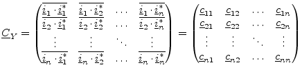 |
(2.36) |
This definition is very likely the one made by eq. (2.1). The matrix has the same properties as well. Because in most transistor models the noise behaviour is expressed as the sum of effects of noise current sources it is easier to form this matrix representation.
Each element in the diagonal matrix is equal to the sum of the noise current of each element connected to the corresponding node. So the first diagonal element is the sum of noise currents connected to node 1, the second diagonal element is the sum of noise currents connected to node 2, and so on.
The off diagonal elements are the negative noise current of the element connected to the pair of corresponding node. Therefore a noise current source between nodes 1 and 2 goes into the matrix at location (1,2) and locations (2,1).
If a noise current source is grounded, it will only have contribute to one entry in the noise correlation matrix - at the appropriate location on the diagonal. If it is ungrounded it will contribute to four entries in the matrix - two diagonal entries (corresponding to the two nodes) and two off-diagonal entries.
Once having defined the spectral noise current densities of the noise
currents within a transistor model the above rules for forming the
![]() matrix can be applied to the example circuit
depicted in fig. 2.5. The noise current
correlation matrix is accordingly
matrix can be applied to the example circuit
depicted in fig. 2.5. The noise current
correlation matrix is accordingly
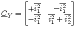 |
(2.37) |
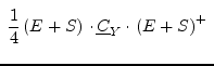
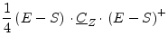
There are three usable noise correlation matrix representations for multiport circuits.
According to Scott W. Wedge and David B. Rutledge [5] the transformations between these representations write as follows.
|
|
|
|
|
|
|
|
|
|
|
|
|
|
|
|
|
 |
 |
|
The signal as well as correlation matrices in impedance and admittance
representations are assumed to be normalized in the above table. ![]() denotes the identity matrix and the
denotes the identity matrix and the ![]() operator indicates the
transposed conjugate matrix (also called adjoint or adjugate).
operator indicates the
transposed conjugate matrix (also called adjoint or adjugate).
Each noise correlation matrix transformation requires the appropriate
signal matrix representation which can be obtained using the formulas
given in section 15.1 on page
![[*]](crossref.png) .
.
![\includegraphics[width=8cm]{CYexample}](img248.png)