Integration methods

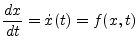
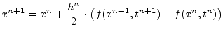
The following differential equation is going to be solved.

$$\dfrac{d x}{d t} = \dot{x}(t) = f(x,t)$$ (6.3)

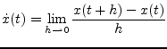
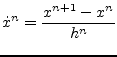
This differential equation is transformed into an algorithm-dependent finite difference equation by quantizing and replacing

$$\dot{x}(t) = \lim_{h \rightarrow 0} \dfrac{x(t+h) - x(t)}{h}$$ (6.4)

by the following equation.

$$\dot{x}^n = \dfrac{x^{n+1} - x^{n}}{h^{n}}$$ (6.5)

There are several linear single- and multi-step numerical integration methods available, each having advantages and disadvantages concerning aspects of stability and accuracy. Integration methods can also be classified into implicit and explicit methods. Explicit methods are inexpensive per step but limited in stability and therefore not used in the field of circuit simulation to obtain a correct and stable solution. Implicit methods are more expensive per step, have better stability and therefore suitable for circuit simulation.

Properties of numerical integration methods

Beforehand some definitions and explanations regarding the terms often used in the following sections are made in order to avoid bigger confusions later on.

• step size
  The step size is defined by the arguments difference of successive solution vectors, i.e. the time step $h^n$ during transient analysis with $n$ being the $n$-th integration step.

  $$h^n = t^{n+1} - t ^n$$ (6.6)

  
  

• order
  The order $k$ of an integration method is defined as follows: With two successive solution vectors $x^{n+1}$ and $x^{n}$ given, the successor $x^{n+1}$ can be expressed by $x^{n}$ by a finite Taylor series. The order of an integrations method equals the power of the step size up to which the approximate solution of the Taylor series differs less than $x^{n}$ from the true solution $x^{n+1}$.

• truncation error
  The truncation error $\varepsilon_T$ depends on the order $k$ of the integration method and results from the remainder term of the Taylor series.

• stability
  In order to obtain an accurate network solution integration methods are required to be stable for a given step size $h$. Various stability definitions exist. This property is explained more in detail in the following sections. Basically it determines the usability of an integration algorithm.

• single- and multistep methods
  Single step methods only use $x^n$ in order to calculate $x^{n+1}$, multi step methods use $x^i$ with $0 \le i < n$.

• implicit and explicit methods
  When using explicit integration methods the evaluation of the integration formula is sufficient for each integration step. With implicit methods at hand it is necessary to solve an equation system (with non-linear networks a non-linear equation system) because for the calculation of $x^{n+1}$, apart from $x^n$ and $\dot{x}^n$, also $\dot{x}^{n+1}$ is used. For the transient analysis of electrical networks the implicit methods are better qualified than the explicit methods.

Elementary Methods

Implicit Euler Method (Backward Euler)

In the implicit Euler method the right hand side of eq. (6.3) is substituted by $f(x^{n+1}, t^{n+1})$ which yields

$$f(x,t) = f(x^{n+1}, t^{n+1}) \;\;\;\; \rightarrow \;\;\;\; x^{n+1} = x^n + h^n\cdot f(x^{n+1}, t^{n+1})$$ (6.7)

The backward euler integration method is a first order single-step method.

Explicit Euler Method (Forward Euler)

In the explicit Euler method the right hand side of eq. (6.3) is substituted by $f(x^{n}, t^{n})$ which yields

$$f(x,t) = f(x^n, t^n) \;\;\;\; \rightarrow \;\;\;\; x^{n+1} = x^n + h^n\cdot f(x^n, t^n)$$ (6.8)

The explicit Euler method has stability problems. The step size is limited by stability. In general explicit time marching integration methods are not suitable for circuit analysis where computation with large steps may be necessary when the solution changes slowly (i.e. when the accuracy does not require small steps).

Trapezoidal method

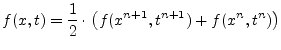
For the bilinear (also called trapezoidal) integration method $f(x,t)$ is substituted by

$$f(x,t) = \dfrac{1}{2}\cdot \left(f(x^{n+1}, t^{n+1}) + f(x^{n}, t^{n})\right)$$ (6.9)

which yields

$$x^{n+1} = x^n + \dfrac{h^n}{2}\cdot \left(f(x^{n+1}, t^{n+1}) + f(x^{n}, t^{n})\right)$$ (6.10)

In each integration step the average value of the intervals beginning and end is taken into account. The trapezoidal rule integration method is a second order single-step method. There is no more accurate second order integration method than the trapezoidal method.

forward-euler

backward-euler

trapezoidal

Linear Multistep Methods

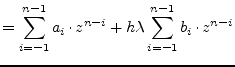
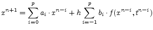
For higher order multi-step integration methods the general purpose method of resolution for the equation $\dot{x} = f(x,t)$

$$x^{n+1} = \sum^p_{i=0} a_i\cdot x^{n-i} + h \sum^p_{i=-1} b_i\cdot f(x^{n-i}, t^{n-i})$$ (6.11)

is used. With $b_{-1} = 0$ the method is explicit and therefore not suitable for obtaining the correct and stable solution. When $b_{-1} \ne 0$ the method is implicit and suitable for circuit simulation, i.e. suitable for solving stiff problems. For differential equation systems describing electrical networks the eigenvalues strongly vary. These kind of differential equation systems are called stiff.

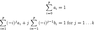
For a polynom of order $k$ the number of required coefficients is

$$2p + 3 \ge k + 1$$ (6.12)

The $2p +3$ coeffcients are choosen to satisfy

$$x^{n+1} = x(t^{n+1})$$ (6.13)

This can be achieved by the following equation system

$$\begin{split}\sum^p_{i=0} a_i = 1\\ \sum^p_{i=1} (-i)^j a_i +... ...} (-i)^{j-1} b_i = 1 & \textrm{ for } j = 1\ldots k \end{split}$$ (6.14)

The different linear multistep integration methods which can be constructed by the equation system (6.14) vary in the equality condition corresponding with (6.12) and the choice of coefficients which are set to zero.

Gear

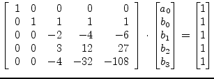
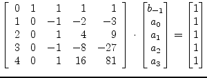
The Gear [7] formulae (also called BDF - backward differentiation formulae) have great importance within the multi-step integration methods used in transient analysis programs. The conditions

$$p = k - 1 \;\;\;\; \textrm{ and } \;\;\;\; b_0 = b_1 = \ldots = b_{k-1} = 0$$ (6.15)

due to the following equation system

$$\left[\begin{array}{lrrrr} 0 & 1 & 1 & 1 & 1\\ 1 & 0 & -1 & -2 & ... ...\\ a_2\\ a_3\\ \end{bmatrix} = \begin{bmatrix}1\\ 1\\ 1\\ 1\\ 1\\ \end{bmatrix}$$ (6.16)

for the Gear formulae of order $4$. Order $k = 1$ yields the implicit Euler method. The example given in the equation system (6.16) results in the following integration formula.

$$\begin{split}x^{n+1} &= a_0\cdot x^{n} + a_1\cdot x^{n-1} + a... ...3} + h\cdot \dfrac{12}{25}\cdot f(x^{n+1}, t^{n+1}) \end{split}$$ (6.17)

There is no more stable second order integration method than the Gear's method of second order. Only implicit Gear methods with order $k \le 6$ are zero stable.

Adams-Bashford

The Adams-Bashford algorithm is an explicit multi-step integration method whence

$$p = k - 1 \;\;\;\; \textrm{ and } \;\;\;\; a_1 = a_2 = \ldots = a_{k-1} = 0 \;\;\;\; \textrm{ and } \;\;\;\; b_{-1} = 0$$ (6.18)

is set to satisfy the equation system (6.14). The equation system of the Adams-Bashford coefficients of order 4 is as follows.

$$\left[\begin{array}{lrrrr} 1 & 0 & 0 & 0 & 0\\ 0 & 1 & 1 & 1 & 1\... ...\\ b_2\\ b_3\\ \end{bmatrix} = \begin{bmatrix}1\\ 1\\ 1\\ 1\\ 1\\ \end{bmatrix}$$ (6.19)

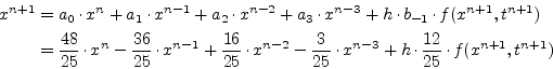
This equation system results in the following integration formula.

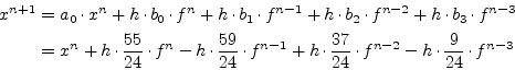$$\begin{split}x^{n+1} &= a_0\cdot x^{n} + h\cdot b_{0}\cdot f^... ...\cdot f^{n-2} - h\cdot \dfrac{9}{24}\cdot f^{n-3}\\ \end{split}$$ (6.20)

The Adams-Bashford formula of order 1 yields the (explicit) forward Euler integration method.

Adams-Moulton

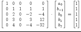
The Adams-Moulton algorithm is an implicit multi-step integration method whence

$$p = k - 2 \;\;\;\; \textrm{ and } \;\;\;\; a_1 = a_2 = \ldots = a_{k-2} = 0$$ (6.21)

is set to satisfy the equation system (6.14). The equation system of the Adams-Moulton coefficients of order 4 is as follows.

$$\left[\begin{array}{lrrrr} 1 & 0 & 0 & 0 & 0\\ 0 & 1 & 1 & 1 & 1\... ...\\ b_1\\ b_2\\ \end{bmatrix} = \begin{bmatrix}1\\ 1\\ 1\\ 1\\ 1\\ \end{bmatrix}$$ (6.22)

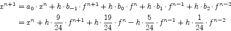
This equation system results in the following integration formula.

$$\begin{split}x^{n+1} &= a_0\cdot x^{n} + h\cdot b_{-1}\cdot f... ...\cdot f^{n-1} + h\cdot \dfrac{1}{24}\cdot f^{n-2}\\ \end{split}$$ (6.23)

The Adams-Moulton formula of order 1 yields the (implicit) backward Euler integration method and the formula of order 2 yields the trapezoidal rule.

Stability considerations

When evaluating the numerical formulations given for both implicit and explicit integration formulas once rounding errors are unavoidable. For small values of $h$ the evaluation must be repeated very often and thus the rounding error possibly accumulates. With higher order algorithms it is possible to enlarge the step width and thereby reduce the error accumulation.

On the other hand it is questionable whether the construction of implicit algorithms is really valuable because of the higher computation effort caused by the necessary iteration (indices $~^{n+1}$ on both sides of the equation). In practice there is a class of differential equations which can be reasonably handled by implicit algorithms where explicit algorithms completely fail because of the impracticable reduction of the step width. This class of differential equations are called stiff problems. The effect of stiffness causes for small variations in the actual solution to be computed very large deviations in the solution which get damped.

The numerical methods used for the transient analysis are required to be stiffly stable and accurate as well. The regions requirements in the complex plane are visualized in the following figure.

Figure 6.1: stability requirements for stiff differential equation systems

For values of $h\lambda$ in region II the numerical method must be stable and accurate, in region I accurate and in region III only stable. The area outside the specified regions are of no particular interest.

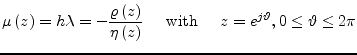
For the stability prediction of integration algorithms with regard to nonlinear differential equations and equation systems the simple and linear test differential equation

$$\dot{x} = \lambda x \;\;\;\; \textrm{ with } \;\;\;\; \lambda \in \mathbb{C}, \left\{\lambda\right\} < 0, x \ge 0$$ (6.24)

is used. The condition Re$\left\{\lambda\right\} < 0$ ensures the solution to be decreasing. The general purpose method of resolution given in (6.11) can be solved by the polynomial method setting

$$x^k = z^k \;\;\;\; \textrm{ with } \;\;\;\; z \in \mathbb{C}$$ (6.25)

Thus we get the characteristic polynom

$$\varphi\left(z\right) = \varrho\left(z\right) + h\lambda \cdot \eta\left(z\right) = 0$$ (6.26)

$$= \sum^{n-1}_{i=-1} a_i\cdot z^{n-i} + h\lambda \sum^{n-1}_{i=-1} b_i\cdot z^{n-i}$$ (6.27)

Because of the conditions defined by (6.14) the above eq. (6.26) can only be true for

$$\left\vert z\right\vert < 1$$ (6.28)

which describes the inner unity circle on the complex plane. In order to compute the boundary of the area of absolute stability it is necessary to calculate

$$\mu\left(z\right) = h\lambda = -\dfrac{\varrho\left(z\right)}{\et... ... \;\;\;\; \textrm{ with } \;\;\;\; z = e^{j\vartheta}, 0 \le \vartheta \le 2\pi$$ (6.29)

These equations describe closed loops. The inner of these loops describe the area of absolute stability. Because $\lambda \le 0$ and $h \ge 0$ only the left half of the complex plane is of particular interest. An integration algorithm is call zero-stable if the stability area encloses $\mu = 0$. Given this condition the algorithm is as a matter of principle usable, otherwise not. If an algorithms stability area encloses the whole left half plane it is called A-stable. A-stable algorithms are stable for any $h$ and all $\lambda < 0$. Any other kind of stability area introduces certain restrictions for $\mu$.

Figure 6.2: areas of absolute stability for order 1...6 Gear formulae

Figure 6.3: areas of absolute stability for order 1...6 Adams-Moulton formulae

Figure 6.4: areas of absolute stability for order 1...6 Adams-Bashford formulae

The figures 6.2, 6.3 and 6.4 visualize the evaluation of eq. (6.29) for the discussed integration methods. All of the implicit formulae are zero-stable, thus principally usable. The (implicit) backward Euler, Gear order 2 and the trapezoidal integration methods are A-stable. Fig. 6.2 shows why the Gear formulae are of such great importance for the transient analysis of electrical networks. With least restrictions for $\mu$ they can be stabilized.