![[*]](crossref.png) ff. various integration methods have
been discussed. The elementary as well as linear multistep methods
(in order to get more accurate methods) always assumed
ff. various integration methods have
been discussed. The elementary as well as linear multistep methods
(in order to get more accurate methods) always assumed
In section 6.1 on pages
ff. various integration methods have
been discussed. The elementary as well as linear multistep methods
(in order to get more accurate methods) always assumed
![]() in its general form. Explicit methods were encountered by
in its general form. Explicit methods were encountered by
![]() and implicit methods by
and implicit methods by
![]() . Implicit methods have been
shown to have a limited area of stability and explicit methods to have
a larger range of stability. With increasing order
. Implicit methods have been
shown to have a limited area of stability and explicit methods to have
a larger range of stability. With increasing order ![]() the linear
multistep methods interval of absolute stability (intersection of the
area of absolute stability in the complex plane with the real axis)
decreases except for the implicit Gear formulae.
the linear
multistep methods interval of absolute stability (intersection of the
area of absolute stability in the complex plane with the real axis)
decreases except for the implicit Gear formulae.
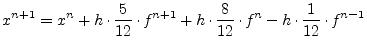
For these given reasons implicit methods can be used to obtain solutions of ordinary differential equation systems describing so called stiff problems. Now considering e.g. the implicit Adams-Moulton formulae of order 3
clarifies that ![]() is necessary to calculate
is necessary to calculate ![]() (and the
other way around as well). Every implicit integration method has this
particular property. The above equation can be solved using
iteration. This iteration is said to be convergent if the integration
method is consistent and zero-stable. A linear multistep method that
is at least first-order is called a consistent method. Zero-stability
and consistency are necessary for convergence. The converse is also
true.
(and the
other way around as well). Every implicit integration method has this
particular property. The above equation can be solved using
iteration. This iteration is said to be convergent if the integration
method is consistent and zero-stable. A linear multistep method that
is at least first-order is called a consistent method. Zero-stability
and consistency are necessary for convergence. The converse is also
true.
The iteration introduces a second index ![]() .
.
This iteration will converge for an arbitrary initial guess
![]() only limited by the step size
only limited by the step size ![]() . In practice successive
iterations are processed unless
. In practice successive
iterations are processed unless
| (6.32) |
The disadvantage for this method is that the number of iterations
until it converges is unknown. Alternatively it is possible to use a
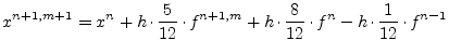
fixed number of correction steps. A cheap way of providing a good
initial guess ![]() is using an explicit integration method,
e.g. the Adams-Bashford formula of order 3.
is using an explicit integration method,
e.g. the Adams-Bashford formula of order 3.
Equation (6.33) requires no iteration process and can be used to obtain the initial guess. The combination of evaluating a single explicit integration method (the predictor step) in order to provide a good initial guess for the successive evaluation of an implicit method (the corrector step) using iteration is called predictor-corrector method. The motivation using an implicit integration method is its fitness for solving stiff problems. The explicit method (though possibly unstable) is used to provide a good initial guess for the corrector steps.
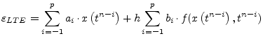
The order of an integration method results from the truncation error
![]() which is defined as
which is defined as
| (6.34) |
meaning the deviation of the exact solution
![]() from the approximate solution
from the approximate solution ![]() obtained by the integration
method. For explicit integration methods with
obtained by the integration
method. For explicit integration methods with
![]() the local
truncation error
the local
truncation error
![]() yields
yields
| (6.35) |
and for implicit integration methods with
![]() it is
it is
| (6.36) |
Going into equation (6.11) and setting
![]() the truncation error is defined as
the truncation error is defined as
With the Taylor series expansions
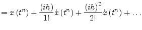 |
(6.38) | |
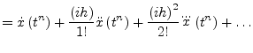 |
(6.39) |
the local truncation error as defined by eq. (6.37) can be written as
| (6.40) |
The error terms ![]() ,
, ![]() and
and ![]() in their general form can then
be expressed by the following equation.
in their general form can then
be expressed by the following equation.
A linear multistep integration method is of order ![]() if
if
| (6.42) |
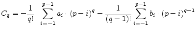
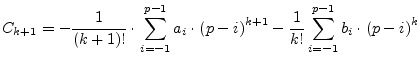
The error constant ![]() of an
of an ![]() -step integration method of
order
-step integration method of
order ![]() is then defined as
is then defined as
 |
(6.43) |
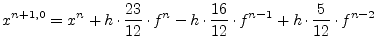
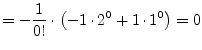
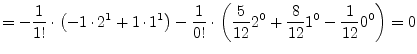
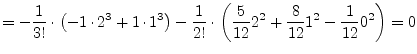
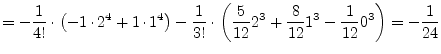
The practical computation of these error constants is now going to be
explained using the Adams-Moulton formula of order 3 given by
eq. (6.30). For this third order method with
![]() ,
,
![]() ,
,
![]() ,
, ![]() and
and ![]() the following
values are obtained using eq. (6.41).
the following
values are obtained using eq. (6.41).
 |
(6.44) | |
 |
(6.45) | |
 |
(6.46) | |
 |
(6.47) | |
 |
(6.48) |
In similar ways it can be verified for each of the discussed linear multistep integration methods that
| (6.49) |
The following table summarizes the error constants for the implicit Gear formulae (also called BDF - backward differention formulae).
| implicit Gear formulae (BDF) | ||||||
|
|
1 | 2 | 3 | 4 | 5 | 6 |
|
|
1 | 2 | 3 | 4 | 5 | 6 |
| error constant |
|
|
|
|
|
 |
The following table summarizes the error constants for the explicit Gear formulae.
| explicit Gear formulae | ||||||
|
|
2 | 3 | 4 | 5 | 6 | 7 |
|
|
1 | 2 | 3 | 4 | 5 | 6 |
| error constant |
|
|||||
The following table summarizes the error constants for the explicit Adams-Bashford formulae.
| explicit Adams-Bashford | ||||||
|
|
1 | 2 | 3 | 4 | 5 | 6 |
|
|
1 | 2 | 3 | 4 | 5 | 6 |
| error constant |
|
|
|
 |
|
|
The following table summarizes the error constants for the implicit Adams-Moulton formulae.
| implicit Adams-Moulton | ||||||
|
|
1 | 1 | 2 | 3 | 4 | 5 |
|
|
1 | 2 | 3 | 4 | 5 | 6 |
| error constant |
|
|
|
|
 |
 |
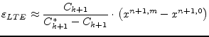
The locale truncation error of the predictor of order ![]() may be
defined as
may be
defined as
| (6.50) |
and that of the corresponding corrector method of order ![]()
| (6.51) |
If a predictor and a corrector method with same orders ![]() are
used the locale truncation error of the predictor-corrector method
yields
are
used the locale truncation error of the predictor-corrector method
yields
 |
(6.52) |
This approximation is called Milne's estimate.
For all numerical integration methods used for the transient analysis of electrical networks the choice of a proper step-size is essential. If the step-size is too large, the results become inaccurate or even completely wrong when the region of absolute stability is left. And if the step-size is too small the calculation requires more time than necessary without raising the accuracy. Usually a chosen initial step-size cannot be used overall the requested time of calculation.
Basically a step-size ![]() is chosen such that
is chosen such that
| (6.53) |
Forming a step-error quotient
| (6.54) |
yields the following algorithm for the step-size control. The initial
step size ![]() is chosen sufficiently small. After each integration
step every step-error quotient gets computed and the largest
is chosen sufficiently small. After each integration
step every step-error quotient gets computed and the largest ![]() is then checked.
is then checked.
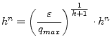
If
![]() , then a reduction of the current step-size is
necessary. As new step-size the following expression is used
, then a reduction of the current step-size is
necessary. As new step-size the following expression is used
 |
(6.55) |
with ![]() denoting the order of the corrector-predictor method and
denoting the order of the corrector-predictor method and
![]() (e.g.
(e.g.
![]() . If necessary the process must
be repeated.
. If necessary the process must
be repeated.
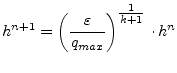
If
![]() , then the calculated value in the current step gets
accepted and the new step-size is
, then the calculated value in the current step gets
accepted and the new step-size is
 |
(6.56) |