![[*]](crossref.png) ) of the transient
simulation. That is why an interpolation of exact values (voltage or
current) at a given point in time is necessary.
) of the transient
simulation. That is why an interpolation of exact values (voltage or
current) at a given point in time is necessary.
The time-domain simulation of components defined in the frequency-domain can be performed using an inverse Fourier transformation of the Y-parameters of the component (giving the impulse response) and an adjacent convolution with the prior node voltages (or branch currents) of the component.
This requires a memory of the node voltages and branch currents for
each component defined in the frequency-domain. During a transient
simulation the time steps are not equidistant and the maximum required
memory length ![]() of a component may not correspond with the
time grid produced by the time step control (see section
6.2.3 on page ) of the transient
simulation. That is why an interpolation of exact values (voltage or
current) at a given point in time is necessary.
of a component may not correspond with the
time grid produced by the time step control (see section
6.2.3 on page ) of the transient
simulation. That is why an interpolation of exact values (voltage or
current) at a given point in time is necessary.
Components defined in the frequency-domain can be divided into two major classes.
Components with constant delay times are a special case. The impulse response corresponds to the node voltages and/or branch currents at some prior point in time optionally multiplied with a constant loss factor.
With no constant delay time the MNA matrix entries of a voltage
controlled current source is determined by the following equations
according to the node numbering in fig. 9.8 on page
.
The equations yield the following MNA entries during the transient analysis.
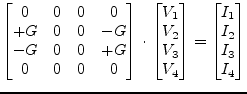 |
(6.109) |
With a constant delay time ![]() eq. (6.108) rewrites as
eq. (6.108) rewrites as
which yields the following MNA entries during the transient analysis.
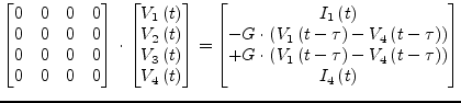 |
(6.111) |
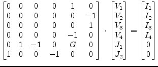
The MNA matrix entries of a voltage controlled voltage source are
determined by the following characteristic equation according to the
node numbering in fig. 9.10 on page .
This equation yields the following augmented MNA matrix entries with a single extra branch equation.
 |
(6.113) |
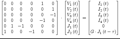
When considering an additional constant time delay ![]() eq. (6.112) must be rewritten as
eq. (6.112) must be rewritten as
This representation requires a change of the MNA matrix entries which now yield the following matrix equation.
 |
(6.115) |
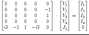
With no time delay the MNA matrix entries of a current controlled
current source are determined by the following equations according to
the node numbering in fig. 9.9 on page .
| (6.116) | ||
| (6.117) |
These equations yield the following MNA matrix entries using a single extra branch equation.
 |
(6.118) |
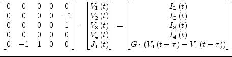
When additional considering a constant delay time ![]() eq. (6.116) must be rewritten as
eq. (6.116) must be rewritten as
Thus the MNA matrix entries change as well yielding
 |
(6.120) |
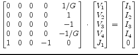
The MNA matrix entries for a current controlled voltage source are
determined by the following characteristic equations according to the
node numbering in fig. 9.11 on page .
| (6.121) | ||
| (6.122) |
These equations yield the following MNA matrix entries.
 |
(6.123) |
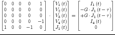
With an additional time delay ![]() between the input current and
the output voltage eq. (6.121) rewrites as
between the input current and
the output voltage eq. (6.121) rewrites as
Due to the additional time delay the MNA matrix entries must be rewritten as follows
 |
(6.125) |
The A-parameters of a transmission line (see eq (9.196) on
page ) are defined in the frequency domain. The
equation system formed by these parameters write as
| (6.126) | ||
 |
(6.127) |
Applying
![]() and
and
![]() to the above equation system and using the
following transformations
to the above equation system and using the
following transformations
 |
(6.128) | |
 |
(6.129) |
yields
whereas ![]() denotes the propagation constant
denotes the propagation constant
![]() ,
,
![]() the length of the transmission line and
the length of the transmission line and ![]() the line impedance.
the line impedance.
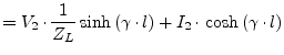
These equations can be transformed from the frequency domain into the
time domain using the inverse Fourier transformation. The frequency
independent loss
![]() gives the constant
factor
gives the constant
factor
| (6.132) |
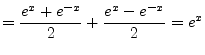
The only remaining frequency dependent term is
| (6.133) |
which yields the following transformation
| (6.134) |
All the presented time-domain models with a frequency-independent
delay time are based on this simple transformation. It can be applied
since the phase velocity
![]() is not a
function of the frequency. This is true for all non-dispersive
transmission media, e.g. air or vacuum. The given transformation can
now be applied to the eq. (6.130) and eq. (6.131)
defined in the frequency-domain to obtain equations in the
time-domain.
is not a
function of the frequency. This is true for all non-dispersive
transmission media, e.g. air or vacuum. The given transformation can
now be applied to the eq. (6.130) and eq. (6.131)
defined in the frequency-domain to obtain equations in the
time-domain.
The length ![]() of the memory needed by the ideal transmission
line can be easily computed by
of the memory needed by the ideal transmission
line can be easily computed by
 |
(6.135) |
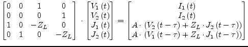
The MNA matrix for a lossy (or lossless with
![]() )
transmission line during the transient analysis is augmented by two
new rows and columns in order to consider the following branch
equations.
)
transmission line during the transient analysis is augmented by two
new rows and columns in order to consider the following branch
equations.
Thus the MNA matrix entries can be written as
 |
(6.138) |
with ![]() denoting the loss factor derived from the constant (and
frequency independent) line attenuation
denoting the loss factor derived from the constant (and
frequency independent) line attenuation ![]() and the transmission
line length
and the transmission
line length ![]() .
.
| (6.139) |
The ideal 4-terminal transmission line is a two-port as well. It differs from the 2-terminal line as shown in fig. 6.5.1 in two new node voltages and branch currents.
The differential mode of the ideal 4-terminal transmission line can be modeled by modifying the branch eqs. (6.136) and (6.137) of the 2-terminal line which yields
| (6.140) | |
| (6.141) |
Two more conventions must be indroduced
| (6.142) | ||
| (6.143) |
which is valid for the differential mode (i.e. the odd mode) of the transmission line and represents a kind of current mirror on each transmission line port.
According to these consideration the MNA matrix entries during transient analysis are
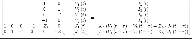 |
(6.144) |
The analogue models of logical (digital) components explained in
section 10.6 on page do not include
delay times. With a constant delay time ![]() the determining
equations for the logical components yield
the determining
equations for the logical components yield
| (6.145) |
With the prior node voltages
![]() known the
MNA matrix entries in eq. (10.268) can be rewritten as
known the
MNA matrix entries in eq. (10.268) can be rewritten as
 |
(6.146) |
during the transient analysis. The components now appear to be simple linear components. The derivatives are not anymore necessary for the Newton-Raphson iterations. This happens to be because the output voltage does not depend directly on the input voltage(s) at exactly the same time point.
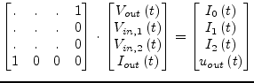
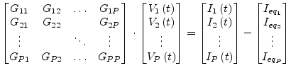
In the general case a component with ![]() ports which is defined in the
frequency-domain can be represented by the following matrix equation.
ports which is defined in the
frequency-domain can be represented by the following matrix equation.
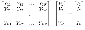 |
(6.147) |
This matrix representation is the MNA representation during the AC analysis. With no specific time-domain model at hand the equation
| (6.148) |
must be transformed into the time-domain using a Fourier transformation.
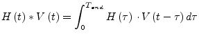
The multiplication in the frequency-domain is equivalent to a convolution in the time-domain after the transformation. It yields the following matrix equation
| (6.149) |
whereas
![]() is the impulse response based on the
frequency-domain model and the
is the impulse response based on the
frequency-domain model and the ![]() operator denotes the convolution
integral
operator denotes the convolution
integral
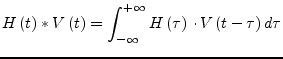 |
(6.150) |
The lower bound of the given integral is set to zero since both the
impulse response as well as the node voltages are meant to deliver no
contribution to the integral. Otherwise the circuit appears to be
unphysical. The upper limit should be bound to a maximum impulse
response time ![]()
with
| (6.152) |
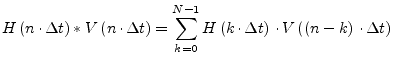
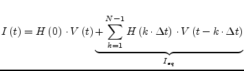
Since there is no analytic represention for the impulse response as well as for the node voltages eq. (6.151) must be rewritten to
with
 |
(6.154) |
whereas ![]() denotes the number of samples to be used during numerical
convolution. Using the current time step
denotes the number of samples to be used during numerical
convolution. Using the current time step
![]() it is
possible to express eq. (6.153) as
it is
possible to express eq. (6.153) as
 |
(6.155) |
With
![]() the resulting MNA matrix equation during
the transient analysis gets
the resulting MNA matrix equation during
the transient analysis gets
| (6.156) |
This means, the component defined in the frequency-domain can be
expressed with an equivalent DC admittance ![]() and additional
independent current sources in the time-domain. Each independent
current source at node
and additional
independent current sources in the time-domain. Each independent
current source at node ![]() delivers the following current
delivers the following current
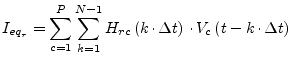 |
(6.157) |
whereas ![]() denotes the node voltage at node
denotes the node voltage at node ![]() at some prior time
and
at some prior time
and ![]() the impulse response of the component based on the
frequency-domain representation. The MNA matrix equation during
transient analysis can thus be written as
the impulse response of the component based on the
frequency-domain representation. The MNA matrix equation during
transient analysis can thus be written as
 |
(6.158) |
With the number of samples ![]() being a power of two it is possible to
use the Inverse Fast Fourier Transformation (IFFT). The
transformation to be performed is
being a power of two it is possible to
use the Inverse Fast Fourier Transformation (IFFT). The
transformation to be performed is
| (6.159) |
The maximum impulse response time of the component is specified by
![]() requiring the following transformation pairs.
requiring the following transformation pairs.
| (6.160) |
with
| (6.161) | ||
 |
(6.162) |
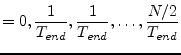
The frequency samples in eq. (6.162) indicate that only
half the values are required to obtain the appropriate impulse
response. This is because the impulse response
![]() is
real valued and that is why
is
real valued and that is why
| (6.163) |
The maximum frequency considered is determined by the maximum impulse
response time ![]() and the number of time samples
and the number of time samples ![]() .
.
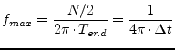 |
(6.164) |
It could prove useful to weight the Y-parameter samples in the frequency-domain by multiplying them with an appropriate windowing function (e.g. Kaiser-Bessel).
For the method presented the Y-parameters of a component must be
finite for
![]() as well as for
as well as for
![]() . To
obtain
. To
obtain
![]() the Y-parameters at
the Y-parameters at ![]() are required.
This cannot be ensured for the general case (e.g. for an ideal
inductor).
are required.
This cannot be ensured for the general case (e.g. for an ideal
inductor).
![\includegraphics[width=0.4\linewidth]{tline}](img672.png)
![\includegraphics[width=0.4\linewidth]{tline4p}](img698.png)