Many simulators support non-ideal transformers (e.g. mutual inductor
in SPICE). An often used model consists of finite inductances and an
imperfect coupling (straw inductance). This model has three
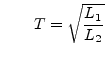
parameters: Inductance of the primary coil ![]() , inductance of the
secondary coil
, inductance of the
secondary coil ![]() and the coupling factor
and the coupling factor ![]() .
.
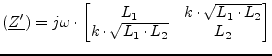
This model can be replaced by the equivalent circuit depicted in figure 9.4. The values are calculated as follows.
 |
(9.42) | |
| (9.43) | ||
| (9.44) | ||
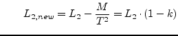 |
(9.45) |
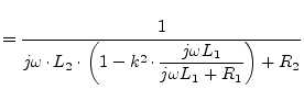
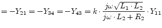
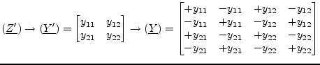
The Y-parameters of this component are:
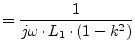 |
(9.46) | |
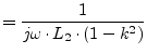 |
(9.47) | |
 |
(9.48) |
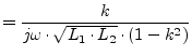
Furthermore, its S-parameters are:
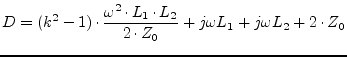 |
(9.49) |
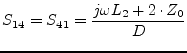 |
(9.50) |
| (9.51) |
 |
(9.52) |
| (9.53) |
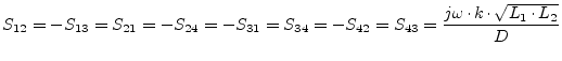 |
(9.54) |
Also including an ohmic resistance ![]() and
and ![]() for each coil,
leads to the following Y-parameters:
for each coil,
leads to the following Y-parameters:
 |
(9.55) | |
 |
(9.56) | |
 |
(9.57) |
Building the S-parameters leads to too large equations. Numerically converting the Y-parameters into S-parameters is therefore recommended.
The MNA matrix entries during DC analysis and the noise correlation matrices of this transformer are:
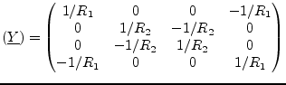 |
(9.58) |
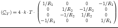 |
(9.59) |
 |
(9.60) |
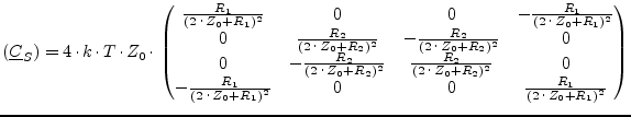
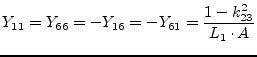
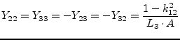
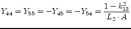
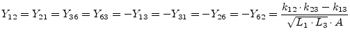
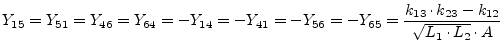
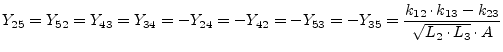
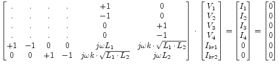
A transformer with three coupled inductors has three coupling factors
![]() ,
, ![]() and
and ![]() . Its Y-parameters write as follows
(port numbers are according to figure 9.3).
. Its Y-parameters write as follows
(port numbers are according to figure 9.3).
| (9.61) | |
 |
(9.62) |
 |
(9.63) |
 |
(9.64) |
 |
(9.65) |
 |
(9.66) |
 |
(9.67) |
A more general approach for coupled inductors can be obtained by using the induction law:
 |
(9.68) |
Realizing this approach with the MNA matrix is straight forward: Every
inductance ![]() needs an additional matrix row. The corresponding
element in the
needs an additional matrix row. The corresponding
element in the ![]() matrix is
matrix is ![]() . If two inductors are
coupled the cross element in the
. If two inductors are
coupled the cross element in the ![]() matrix is
matrix is
![]() . For two coupled inductors this yields:
. For two coupled inductors this yields:
 |
(9.69) |
Obviously, this approach has an advantage: It also works for zero inductances and for unity coupling factors and is extendible for any number of inductors. It has the disadvantage that it enlarges the MNA matrix.
The S-parameter matrix of this component is obtained by converting the Z-parameter matrix of the component. The Z-parameter matrix can be constructed using the following scheme: The self-inductances on the main diagonal and the mutual inductances in the off-diagonal entries.
 |
(9.70) |
This matrix representation does not contain the second terminals of the inductances. That's why the Z-parameter matrix must be converted into the Y-parameter matrix representation which is then extended to contain the additional terminals.
 |
(9.71) |
![\includegraphics[width=7.5cm]{nitrafo}](img927.png)